
Step 1: Open Your Excel File
Start by opening the Excel sheet where you have many columns.
These could be monthly reports, sales data, expenses, or any long horizontal dataset.
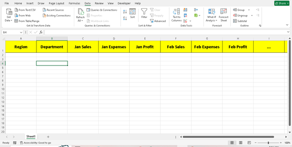
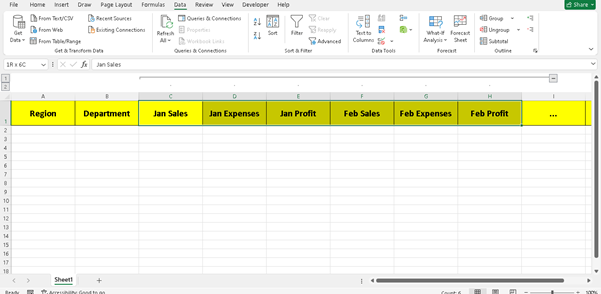
I Have this Type Of Data >
Step 2: Select the Columns You Want to Group
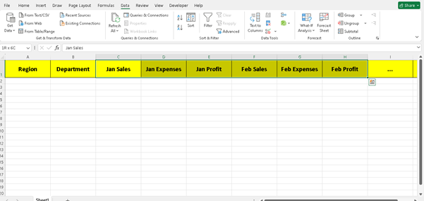
Click and drag to highlight the columns you want to group.
I want To Group from “Jan Sales” to “Feb Profit”.
Hold the Shift key and click the first and last columns to select them quickly.
Step 3: Go to the “Data” Tab
Once your columns are selected, go to the top menu ribbon and click on the “Data” tab.
There, look for the section called “Outline”. Inside it, you’ll find a button named “Group”.
Click The Top Right Group Option and select column
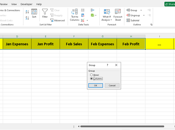
You Get This Type Of Interface
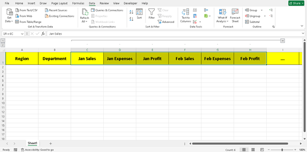
You’ll see a minus sign (-) at the top of the grouped columns.
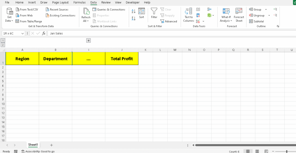
To view the hidden columns again, just click the plus sign (+).
Final Thoughts
That’s it Your Grouping Is Successfull
Thank You