
Step 1: Insert Pivot Table
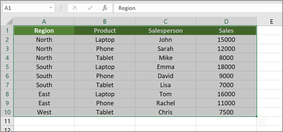
- Select any cell in your data (or the entire range, e.g., A1:D10).
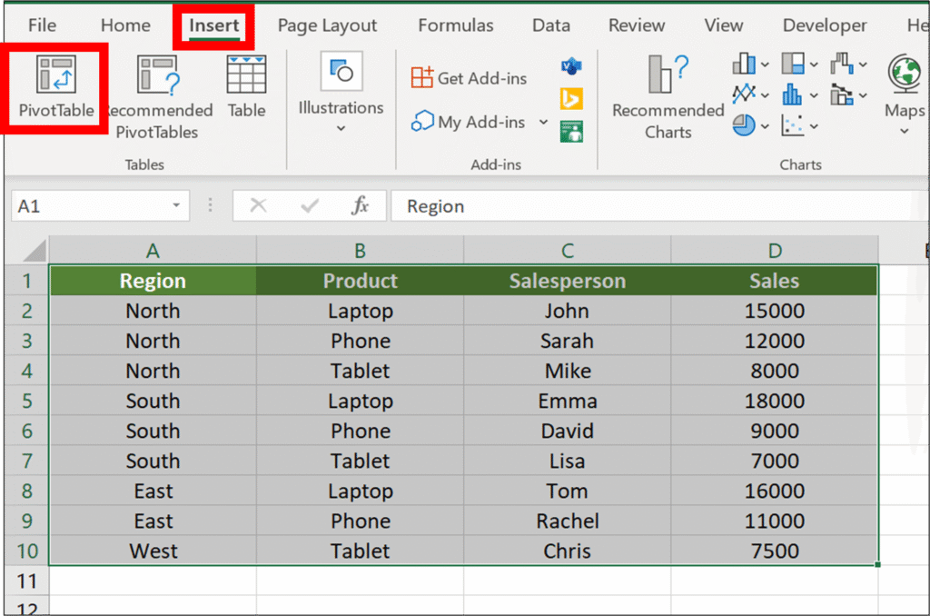
2. Go to Insert → PivotTable.
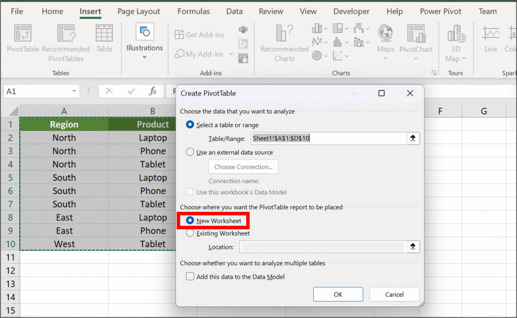
3. Choose New Worksheet (or existing) and click OK.
Step 2: Set Up Pivot Fields
- In the PivotTable Fields pane:
- Drag Region to Rows.
- Drag Product below Region in Rows.
- Drag Salesperson below Product in Rows.
- Drag Sales to Values.
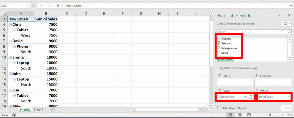
Step 3: Enable Repeated Labels
- Click anywhere inside the pivot table.
- Go to the Design tab (under PivotTable Tools).
- Click Report Layout → Show in Tabular Form.

4. Click Report Layout again → Repeat All Item Labels.
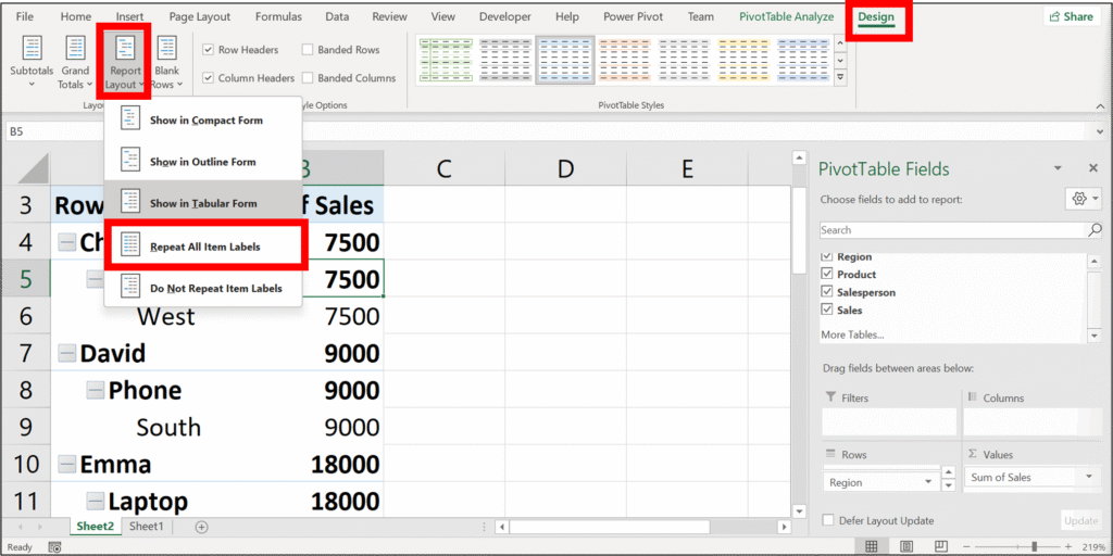
5. Not cleaned yet:
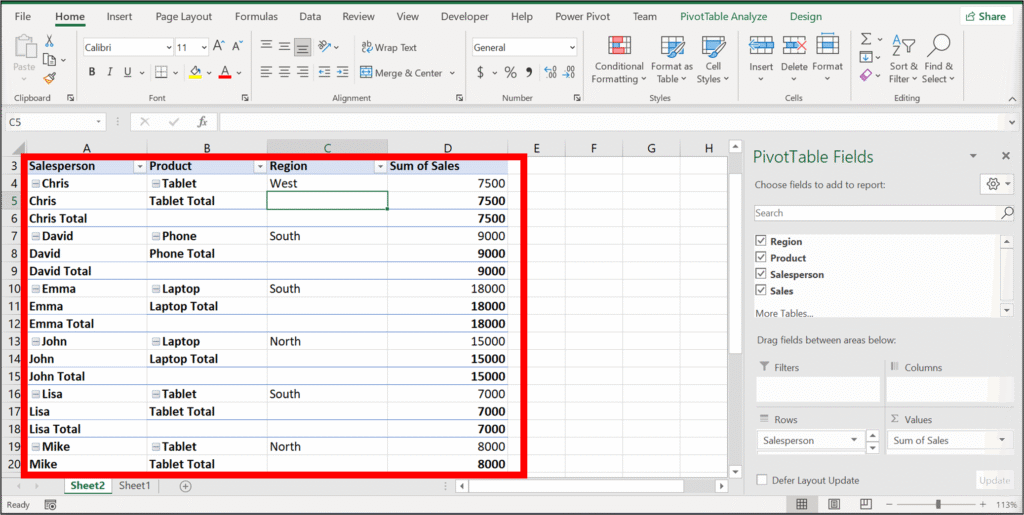
6. Cleaning
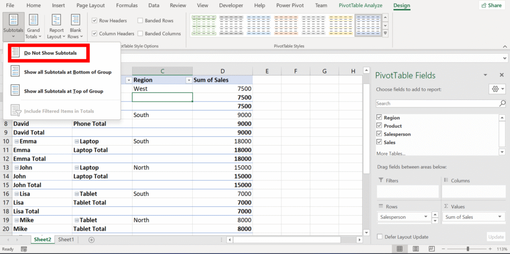
Click on any cell in pivot table and then go to design tab
Click on subtotals and select “DO NOT SHOW SUBTOTAL“
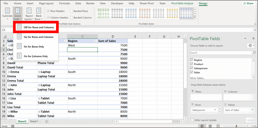
7. Then go to Grand Total and select off for row and column in design tab:
FINAL LOOK:

Hope you liked it! Thanks for reading till the end. We’ll meet again in the next exciting topic