

STEP 1:
Set up your data in the table from which we will retrieve the data.
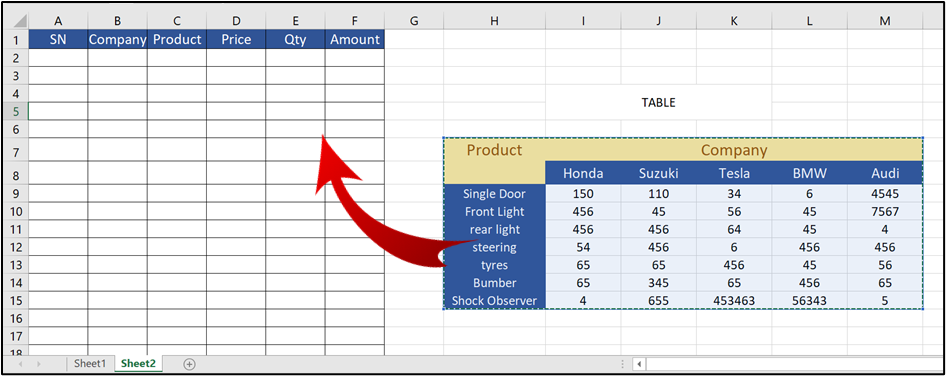
STEP 2:
Add a dropdown in Columns B and C for Company and Product.
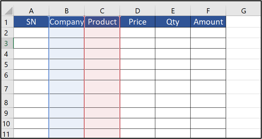
Use the Data Validation tool to add dropdowns. Below are the steps to create a dropdown for Company For Product follow the same method.
1st Step:
select column B for Company then
go to data validation tool from Data tab
new Window Will pop up
select list in allow dropdown
then in source add company names
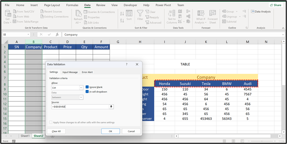
It Look like this:
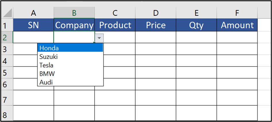
Repeat same Steps for product column:
STEP 3:
Enter the below Formula In D2 For Price
and Drag down
FORMULA: =IFERROR(INDEX($H$8:$M$15, MATCH(C2, $H$8:$H$15, 0), MATCH(B2, $H$8:$M$8, 0)), “”)
FORMULA BREAKDOWN:
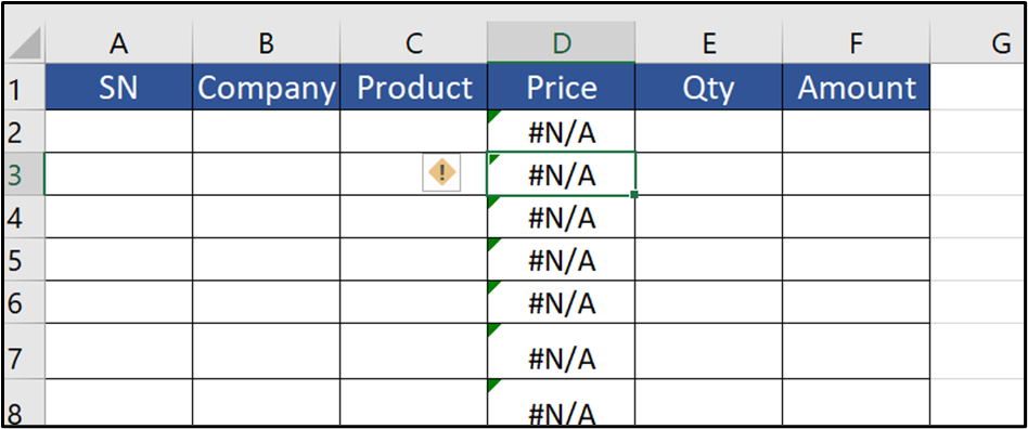
If error to make Clean if there is no content in dropdown if If error is not in dropdown it will look like this:
And Match and Index formula to find row and Column Number from the table
Here is final Look and working:
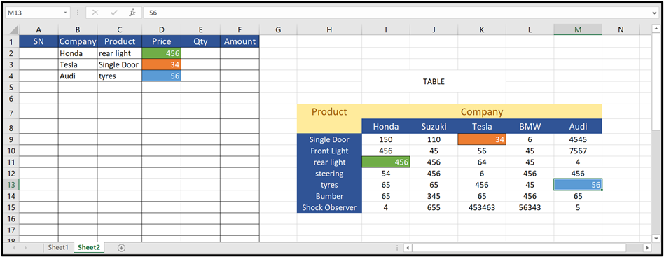
When you choose a company and product from the dropdowns (as shown above), the corresponding price will automatically display in the next cell.
Hope you liked it! Thanks for reading till the end. We’ll meet again in the next exciting topics.
For premium Excel services at affordable prices with guaranteed quality, visit our website:
www.irfanai.com“