
Let’s go through a step-by-step guide to master relative and absolute references.
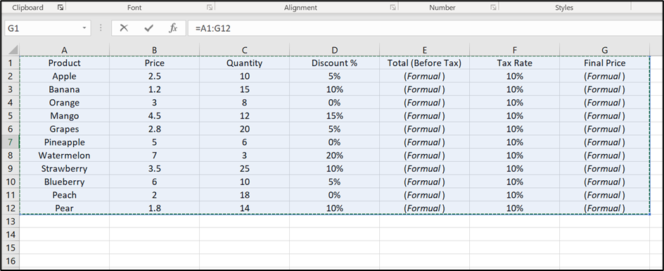
Step 1: Set Up Data
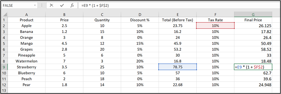
Setup your data in Excel or Google Sheets as shown below:
Step 2: Calculate Total (Before Tax) Using Relative References
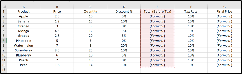
Total = (Price × Quantity) – Discount
- Click on E2 cell.
- Enter the formula.
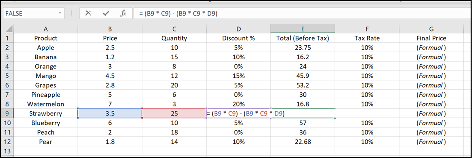
= (B2 * C2) – (B2 * C2 * D2)
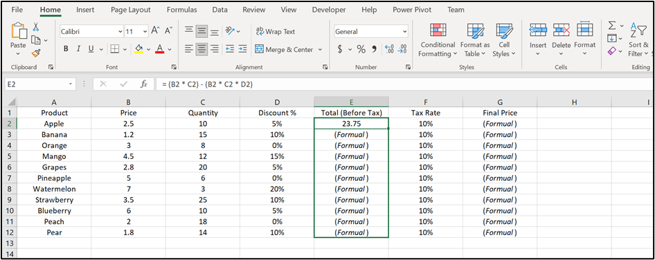
Drag to E12 cell
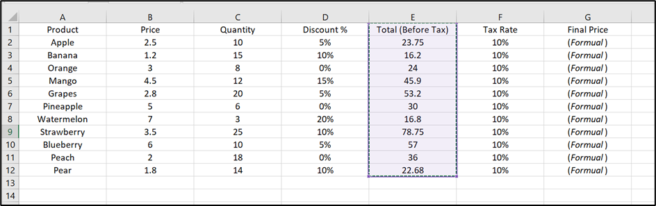
The formula will adjust itself automatically as shown in image and this is called relative reference or addressing.
Step 3: Calculate “Final Price” Using Absolute Reference for Tax Rate
Final Price = Total × (1 + Tax Rate)
Click on G2 cell
Enter the formula:
= E2 * (1 + $F$2)
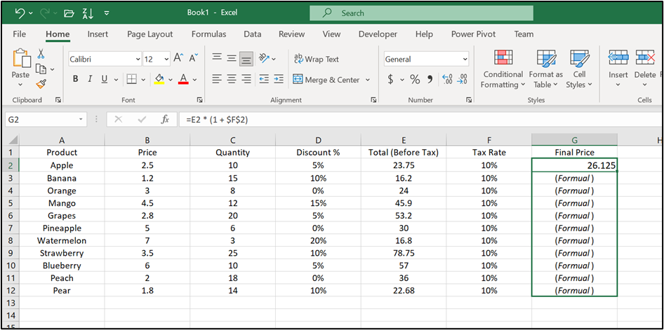
Press Enter, then drag the formula down to G12.
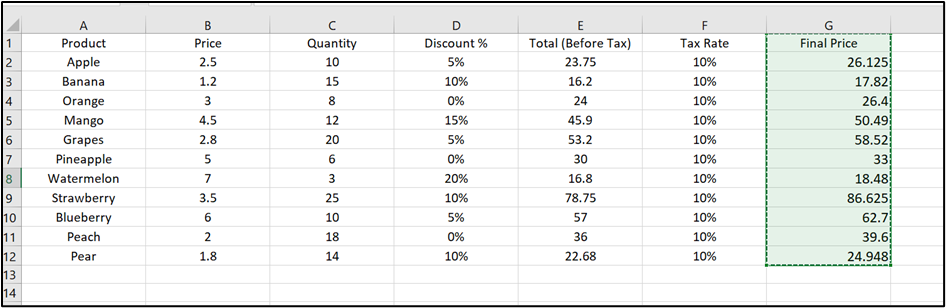
The formula adjusts for E2 and E12 but always uses F2 for tax rate as shown in below Images.
Image 1
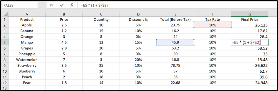
Image 2
So, that’s it! This is how relative and absolute references are used.
Hope you liked it! Thanks for reading till the end. We’ll meet again in the next exciting topic.